
Basic Instructions for Putting Data onto a Standard System
Brian D. Warner, Center for Solar System Studies
For maximum benefit to research, your photometry data should be on or close to a standard system, e.g., Johnson-Cousins BVRcIc or Sloan Digital Sky Survey (SDSS) griz. In other words, the magnitudes you report should be as the objected appeared in the sky if viewed through one of these magnitude bands.
If you have one or more of these filters (available directly from several suppliers or popular on-line astronomical product dealers), the process is straight-forward. Even if you don't, and are working with a clear or no filter, then with some additional care you can provide data reduced to one of the common magnitude bands.
Users of Astrometrica, VPhot (for AAVSO members), or MPO Canopus are probably already familiar with producing sky magnitudes. Therefore, these procedures are aimed mostly at those who have software that can accurately measure the brightness of stars and asteroids on their images, producing what are called "instrumental magnitudes" and need to take the extra steps to convert those instrumental magnitudes into sky magnitudes.
Before getting started, it is important to note that if working an asteroid, there are additional considerations that will be discussed below. In short, these cover additional corrections to the sky magnitudes. It is probably best not to include these corrections but you should be aware of them and how they are computed and applied.
Recommended Reading
What's below summarizes information that you can find in several excellent references on photometry. You're strongly encouraged to read one or more of these at some point so that you can have a much better understanding of photometry.
The Handbook for Astronomical Image Processing (2000). Richard Berry and James Burnell. Willmann-Bell (Includes AIP4WIN software).
Astronomical Photometry: A Text and Handbook for the Advanced Amateur and Professional Astronomer (1990). Arne A. Henden and Ronald H. Kaitchuck. Willmann-Bell.
Handbook of CCD Astronomy, 2nd Edtion (2008). Steve B. Howell. Cambridge University Press.
A Practical Guide to Lightcurve Photometry and Analysis, 2nd Edition (2016). Brian D. Warner. Springer.
AAVSO CCD Observing Manual. Available on-line at: https://www.aavso.org/ccd-camera-photometry-guide
Getting Started
It is presumed that you have software that can measure your images and find a value for each star and target of interest. Usually, this is determined with:
Im = -2.5*log(ADU/Exp)
Where is the Im instrumental magnitude
ADU is the sum of pixel values that are a direct result of the star or target
Exp is the exposure in seconds
The division by the exposure normalizes all values to a common exposure of one second. Therefore, you can directly compare magnitudes of images taken with the same telescope/camera but with different exposures.
Technically, the software should convert the ADU values to electrons using the camera's eADU factor (the number of electrons per unit of ADU). However, all this does is change the result by constant equal to log(eADU), i.e., all instrumental magnitudes with and without the conversion differ by a constant offset. For example, if ADU is 60,000, then Eq. 1 gives -11.945. If the eADU factor is 2.3, then ADU becomes 138000 and Eq. 1 gives -12.850, or a difference of -0.905 which, accounting for rounding, is equal to -2.5*log(2.3).
This value results in a negative number, and so the brighter the object, the more negative the number. Since this is not considered "human friendly", an arbitrary, large number is added to the negative value to get a positive instrumental magnitude. This number is often +25, i.e.,
Im = -2.5*log(ADU/Exp) + 25
and so, assuming a raw instrumental magnitudes of -7.000 and -12.000 (the second star being 5 magnitudes brighter), this gives
Im = -2.5*log(ADU/Exp) + 25.0
Im = -7.000 + 25.000 = 18.000
Im = -12.000 + 25.000 = 13.000
Finding the Instrumental Offset
Let*apos;s call that arbitrary value (+25 above) "instrumental offset" or just "offset."
The simplest way to determine that value is if there is a star in your image with a good catalog value. This can be from the APASS catalog from the AAVSO, the CMC-15 (which will have SDSS r´ magnitudes), or, the recommended ATLAS, also with SDSS magnitudes.
- Take 3-5 images of the field in good conditions (no clouds, haze, etc).
- Measure the raw instrumental magnitude of the reference star
- Find the offset using
Offset = Im + M
Where Im is the instrumental magnitude and M is the catalog magnitude in the color of choice, e.g, Johnson V.
For example, if the instrumental magnitude -7.000 and the catalog magnitude is V = 12.000 then
Offset = -7.000 + 12.000 = +19.000
By rearranging Eq. 3 to solve for M
M = Im + Offset
You can find the catalog magnitude for any object in the image. For example, if the target has an instrumental magnitude of -11.585, then<.p>
M = -11.585 + 19.000 = +7.415
To get more reliable results and to be able to estimate the error of the offset, use several stars to establish the offset value. In this case, you would find the average of the several offsets for the offset value and the standard deviation of the average to estimate the error.
There is a very important caution here: this works only for stars in the single image (or within the small set used to find the offset) and if the reference star and target are similar in color.
The references mentioned above go into more detail why the above works in limited situations. Briefly, the raw instrumental magnitude is dependent on what's call the "air mass", roughly speaking, the path length of the star's light through the Earth's atmosphere. An air mass (X) of 1.00 is for a star that is exactly at the zenith. An approximate definition is
X = sec(z)
Where z is the angular distance of the star from the zenith. A star at the horizon has a zenith distance of 90° and an infinite air mass (not really, of course: the Earth's atmosphere is not infinitely thick).
The issue of color difference has to do with your system's response to a range of colors and how closely that matches the response of the system that defined the standard system to which you're trying to convert. If using a filter, you have a little more freedom in choosing reference (and comparison stars, which will be covered below) since your system's color response will be close to the standard system. However, if working unfiltered, then you need to be sure to use stars very close in color (as determined by the B-V, V-R color index) to your target.
It's Not Quite That Simple
If you're working a variable star or other object that does not move from night to night, you can use the same reference star in the same field of view, but you must determine the offset not only every night but for every image.
What's been described to this point works only if the sky conditions never change after you've determined the offset value. This is never the case. Very thin clouds, rising/lowering humidity, and other things can change the transparency of the sky and so, at any given moment, your reference star will have a different instrumental magnitude.
Even without clouds or haze, as the field rises and falls in the sky during the night, the air mass changes, meaning that as the field rises, all stars in the field get a little brighter and, as the field falls, they get a little fainter. Therefore, in reality, the offset you've found so far is valid for a single moment in time on a given night. This is hardly useful in real-world situations but understanding the process to this point is important before taking the final steps.
To complicate matters, if you're working a moving target such as an asteroid, you will have to use different reference stars every night, meaning you have to hope that there is at least one star in the field with a good catalog magnitude. If the asteroid is moving very fast, you may have to use several references through the course of the night. This makes for more work but the result is that all your data will appear to have used a single reference for all observations.
Differential Photometry to the Rescue
To achieve the goal of finding an accurate catalog (sky) magnitude of the target on every image, you can take advantage of several important facts. First, for relatively small fields (say 30 arcmin/side and less) that are at least 30° above horizon, that the atmospheric extinction measured by the air mass is essentially the same. In this case, the offset value is constant across the field of view. Second, if you use references that are very close in color, you can ignore those corrections. Third, there is the presumption that extinction due to clouds, haze, or changing humidity is also constant across the entire field. Assuming these conditions are true (and they generally are), accurate photometry is well within reach.
First, let's define a new formula that finds the catalog (sky) magnitude of the target.
Mt = (Imt - Imc) + Mc
Where Imt is the instrumental magnitude of the target>
Imc is the instrumental magnitude of a comparison starMc is the catalog magnitude of the comparison star
So, for example,
Mt = (-7.000 - (-9.000)) + 12.000 = (+2.000) + 12.000 = 14.000
Since the instrumental magnitude of the target is 2 magnitudes fainter than the comparison star, the result that catalog magnitude of the target is 2 magnitudes fainter than the catalog magnitude of the comparison is fainter is what's expected.
One comp star is one star away from disaster. What if that star is variable? Then the target magnitudes will vary not only due to its natural causes (e.g., rotation of an asteroid) but the comp star's variations will be superimposed on top of those.
The long-time solution has been to use a "check" star, a second comparison that is treated like a second target. In that case, the check star takes the place of the target. If the two stars are constant (within the errors of the data), then Mt will be (essentially) constant. In fact, you can take the standard deviation of the average of all the check star Mt values as the approximate error of the observations.
Improving the Results
If you use N comparison stars, then you can find the average of Mt for the N results and the standard deviation for the error of each measurement. Using more comparison stars reduces the overall error by sqrt(N). So, if you double the number of comparisons, the error is ~0.71 the error using N/2 stars, assuming good data. This also gives you more room for error should more than one of the comparison stars is variable.
When using multiple comparisons, then for each image, you can treat each comparison star as the check star (Imt in Eq. 6) and use the average of the remaining comparisons (as Imc in Eq. 6) to find the differential value. The result for each comparison should be a constant (not always the same as for the other comparisons) throughout the night.
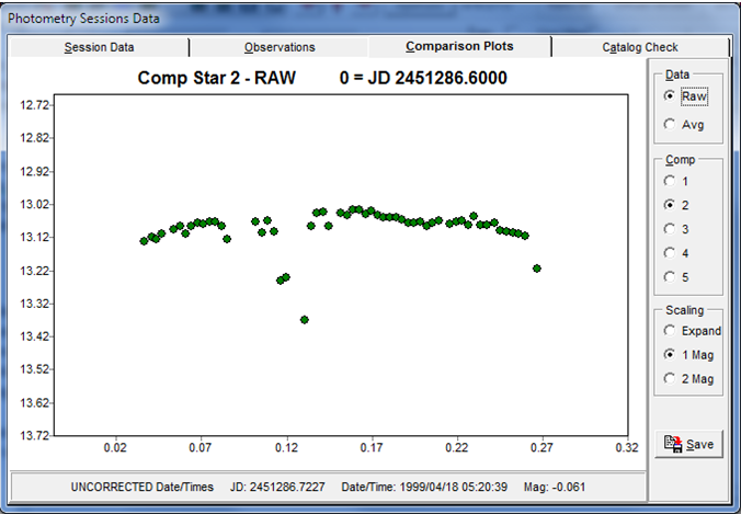
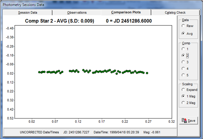
Figure 1. Plots of a comparison stars during an observing session. The left-hand plot shows the raw data. The right-hand plot those the differential value between the comparison and the average of three other comparisons.
In Figure 1, the left-hand screen shot shows a plot of the raw instrumental magnitudes for a comp star (1 of 4) during an observing session. Overall, the slight upward bowing is caused by the extinction decreasing as the field rose higher in the sky, reached the meridian, and then got lower. You can see that there were some thin clouds for a few images, when the star was considerably fainter. The right-hand plot shows why differential photometry is so useful. This gives the differential magnitude between the comparison star and the average of the other three comparisons image-by-image. The standard deviation of the average of all the values was 0.009 mag, meaning that the target observations had approximately this error.
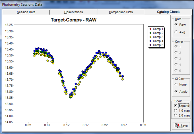
Figure 2. An asteroid's sky magnitudes using differential photometry with five comparison stars.
Figure 2 shows the derived catalog (sky) magnitudes of an asteroid using five comparison stars when applying Eq. 6 for each asteroid-comparison pair. The very tight overlap indicates that 1) the target and stars were of similar color and 2) the catalog magnitudes were internally consistent (close to a standard system).
Asteroids Ahead
All of the above applies equally well to variable targets of any kind, stars, asteroids, whatever. However, when working with asteroids, there's more involved if you want to merge data from several nights to form a composite lightcurve for period analysis.
Before proceeding, note that for best results, all comparison stars should have a "color index" of about 0.7 < B-V < 0.9. Asteroids tend to be slightly redder than the Sun, which is why this range of colors.
As an asteroid orbits the Sun, its distances from the Sun and Earth change. This means that all other things being equal, the asteroid naturally changes brightness over time, getting brighter as it gets closer to Earth, but only if not also getting farther away from the Sun.
To account for changing distances, a correction can be applied
M = -5*log(SunDist * EarthDist) (7)
Where M is the correction in magnitudes to be applied to the computed
catalog ("sky") magnitude
and SunDist and EarthDist are the distances, in au, of the asteroid.
Magnitudes that have been corrected using Eq. 7 are often called "reduced" (not to be confused with the application of photometric corrections) or "corrected for unity distances."
To complicate matters even more, the asteroid's brightness is not dictated by distances alone. When the angle between the Sun and Earth in the sky as seen from the asteroid, the "solar phase angle" is less than about 7° and goes towards 0° (or nearly so) when the asteroid is at opposition, the asteroid's brightness increases beyond what it might otherwise. This is due to what's called the "opposition effect" and has to do with the way the asteroid reflects light when it's coming almost directly perpendicular to the surface.
Both of these corrections must be applied so that the observations can be treated as having been made at a constant phase angle and distances and proper period analysis be done. Otherwise, the period search algorithms will try to account for these variations in addition to those due to rotation.
MPO Canopus applies these corrections as a matter of course. If you are using other software, then you need to determine the corrections and apply them as needed.
However, if you are in working in collaboration with others, do what the lead investigator asks. In most cases, he will ask for magnitudes that are not corrected for these two factors. This way, he can apply the corrections for all data in a consistent way and know exactly what was done.
There is one more correction to be applied before period analysis can begin. This is true for asteroids and variable stars. For asteroids, it is called "light-time correction." As discussed above, an asteroid's distance from Earth is constantly changing. Since light travels at a finite speed, you must correct the timing of the observations so that they are referenced to a fixed distance. This is done by subtracting the light-time from the JD of the observation so that the JD is reference to when the light left the asteroid, not when it arrived at Earth.
Where T is the corrected date, t is the Earth-based date of the observation, and D is the asteroid-Earth distance in au.T = t - D * 0.005778 (days)
For variable stars, the "Heliocentric JD" or "Barycentric JD" is used, which is the time the variable's light reaches the Sun, or for the latter, the gravitational center of the Solar System (a point inside but not at the center of the Sun). See the references above for the formula for this correction.